This is an updating note on random signal analysis.
Random Signal Basic
Review
At first, we should have a prior that to define a random variable, one tool is probability, and the other one is statistics (moment, cumulants).
Probability distribution
In 1D, at first, we have random variable X .
Then we have to describe the relationship between X and its probability distribution.
Culminative Distribution Function (CDF): $ F(x)=p(X \leq x)$
Probability Density Function (PDF): $f(x)=\frac{dF(x)}{dx}$
In 2D, random variable X can be specified as (X,Y)
CDF: $F_{XY}(x, y)=p(X \leq x, Y \leq y)$
PDF: $ \frac{\partial^{2} F_{XY}(x,y)}{\partial x \partial y}$
Marginal Distribution: $f_{X}(x)=\int\limits_{-\infty}^{+\infty} f_{XY}(x,y)dy$
Conditional Distribution: $f_Y(y|x)=\frac{f_{XY}(x,y)}{f_X(x)}$
Moment and Cumulant
In 1D case:
The n-th ordinary moment: $m_n=E[X^n],\ n=1,2,…$
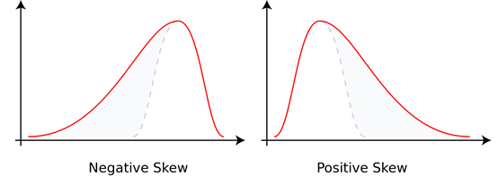
The zeroth moment is the total probability (i.e. one), the first moment is the mean, the second central moment is the variance, the third standardized moment is the skewness, and the fourth standardized moment is the kurtosis. The mathematical concept is closely related to the concept of moment in physics.
For the second and higher moments, the central moment are usually used rather than the moments about zero, because they provide clearer information about the distribution’s shape.
The n-th central moment: $\mu_{n}=E\{(X-E[X])^n\},\ n=1,2,…$
The second central moment $μ_2$ is called the variance, and is usually denoted $σ_2$, where σ represents the standard deviation.
The third and fourth central moments are used to define the standardized moments which are used to define skewness and kurtosis, respectively.
Ordinary moment vs Central moment:
- The 1st ordinary moment is the mean. — Define concentration.
- The 2nd central moment is the variance. — Define dispersion.
- The 3rd central moment is a standardized moment. — Define skewness.
- The 4th central moment is a standardized moment. — Define kurtosis.
Higher moments (>2) are used to describe the deviation from gaussian variables. Only 1~2-th moment are required to analyze gaussian variables because higher moments are relevant to these lower moments.
In 2D case:
- The (n+k)-th mixed ordinary moment: $m_{nk}=E[X^nY^k]$; when n=1, k=1, called relevant moment $R_{XY}$ .
- The (n+k)-th mixed central moment: $\mu_{nk}=E\{(X-E[X])^n(Y-E[Y])^k\}$; when n=1, k=1, called covariance $C_{XY}$
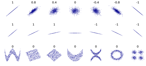
- Correlation Coefficient: $r_{X,Y}=\frac{cov(X,Y)}{\sigma_{X}\sigma_{Y}}$, where $cov(X,Y)$ is the 2nd mixed central moment called covariance and $\sigma$ is standard deviations. It is a measure of the linear correlation between two variables.
- Cumulant: a concept close to moment.
As for gaussian variables, higher moments are determined by lower moments so only 1~2nd moments are necessary. From the perspective of cumulants, when n>2, they are zero in this case. Moreover, if the gaussian variables have zero mean, moments are even the same as cumulants. We can take it easy.
Statistical independence and irrelevance
- Statistical Independence:
- Irrelevance (In short of linear irrelevance): $r_{XY}=0$. We gain $R_{XY}=E[XY]=E[X]E[Y]$. (2nd central moment = 0)
Generally speaking, Statistical Independence $\Rightarrow$ Irrelevance. As for gaussian random variables, Statistical Independence $\Leftrightarrow$ Irrelevance.
- Orthogonality: $R_{XY}=E[XY]=0$ (2nd ordinary moment = 0)
Characteristic function
In probability theory and statistics, the characteristic function of any real-valued random variable completely defines its probability distribution. If a random variable admits a probability density function, then the characteristic function is the Fourier transform of the probability density function. Thus it provides the basis of an alternative route to analytical results compared with working directly with probability density functions or cumulative distribution functions. There are particularly simple results for the characteristic functions of distributions defined by the weighted sums of random variables.
- Characteristic function: $\phi(\omega)=E[e^{j\omega X}]$
The characteristic function is the Fourier transform of the probability density function. (It is not exactly the same, because of $\pm j\omega X$.)
Another feature is that characteristic function is correspond to moment, so characteristic function is also named moment-generating function.
Distribution model
In this part, we have a brief introduction of ordinary distribution models in order to classify our problems into different models.
Easy ones
- Binomial distribution
To be or not to be, that is the question. We have only two choices.
- Poisson distribution
No matter how long I have been waiting for the bus, how many buses will arrive in the coming 5 mins are a constant.
It is a discrete probability distribution that expresses the probability of a given number of events occurring in a fixed interval of time or space if these events occur with a known constant rate and independently of the time since the last event. (Poisson distribution)
- Uniform distribution
There is no bias within the probabilities of different choices.
Gaussian distribution
Detailed information can be found in “Probability theory”.
$\chi^2$ distribution
$\chi^2$ distribution is also named chi-squared distribution.
- Central $\chi^2$ distribution: $Y=\sum_{i=1}^{n}{X_{i}^2}$
It has n degrees of freedom and is the distribution of a sum of the squares of n independent standard normal random variables (Mean=0, variance=1).
- Noncentral $\chi^2$ distribution: $Y=\sum_{i=1}^{n}{X_{i}^2}$
It has n degrees of freedom and is the distribution of a sum of the squares of n independent random variables (Mean=$m_{i}$, variance=$\sigma^2$).
Rayleigh distribution
- Rayleigh distribution: $R=\sqrt{Y}=\sqrt{X^1+X^2}$
It is essentially a central $\chi ^2$ distribution with two degrees of freedom.
- Generalized Rayleigh distribution: $R=\sqrt{Y}=\sqrt{\sum_{i=1}^{n}{X_{i}^2}}$
It is essentially a central $\chi ^2$ distribution with n degrees of freedom.
- Rice distribution: $R=\sqrt{Y}$
It is essentially a noncentral $\chi ^2$ distribution with n degrees of freedom.
Stochastic Process
From random variable to stochastic process
Stochastic process definition
Historically, the random variables were associated with or indexed by a set of numbers, usually viewed as points in time, giving the interpretation of a stochastic process representing numerical values of some system randomly changing over time, such as the growth of a bacterial population, an electrical current fluctuating due to thermal noise, or the movement of a gas molecule. (Stochastic process)
In short, a stochastic process has two dimensions - Time and Value. At a specific time, the value is a random variable. This random variable may be determined by time $t$, which means at another specific time, the random variable may differ.
P.S. Probability distribution and numerical characteristics describe the random variable in the Value axis. There is no random variables along the Time axis but properties of random variables change along the Time axis. 1D means one random variable and 2D means two random variables in different times.
Probability distribution
In 1D (one variable $x$ given one specific time $t$),
CDF: $ F_{X}(x_1,t_1)=P(X(t_1)\leq x_1)$
PDF: $f_X(x_1,t_1)=\frac {\partial F_X(x_1,t_1)}{\partial x_1}$
We can easily find that this stochastic process is a function of x and t.
In 2D (two variable $x$ given two specific time $t$),
CDF: $ F_{X}(x_1,x_2;t_1,t_2)=P\{(X(t_1)\leq x_1, X(t_2)\leq x_2)\}$
PDF: $f_X(x_1,x_2;t_1,t_2)=\frac{\partial ^2 F_X(x_1,x_2;t_1,t_2)}{\partial x_1 \partial x_2}$
It describes the relevance of two moments of the stochastic process, which is widely used in engineering.
Numerical characteristic
In 1D,
- Expectation: $m_X(t)=E[X(t)]=\int\limits_{-\infty}^{+\infty}x f_{X}(x,t)dx$
- Variance: $\sigma^2 _X(t)=D[X(t)]=\int\limits_{-\infty}^{+\infty}[x-m_X(t)]^2 f_{X}(x,t)dx$
The expectation and variance are both definite functions of time t.
In 2D,
- Autocorrelation: $R_X(t_1,t_2)=E[X(t_1)X(t_2)]=\int\limits_{-\infty}^{+\infty}\int\limits_{-\infty}^{+\infty}x_1x_2 f_X(x_1,x_2;t_1,t_2)dx_1dx_2$.
- Cross-correlation: $R_{XY}(t_1,t_2)=E[X(t_1)Y(t_2)]=\int\limits_{-\infty}^{+\infty}\int\limits_{-\infty}^{+\infty}xy f_{XY}(x,y;t_1,t_2)dxdy$.
It is the 2nd mixed ordinary moment of random process. And it describes the relationship of two times.
class note: The usage of autocorrelationIn communication system, autocorrelation of a communication channel can be used to determine whether this channel changes abruptly. If $R_X(t_1,t_2)$ is small, it indicates that this channel changes slowly, vice versa.
Autocorrelation is a square function that describes a linear relationship. It instructs the design of Adaptive differential pulse-code modulation (ADPCM).
Stationary process and ergodicity
Strictly stationary process
This is the definition of n-th strictly stationary process and its PDF doesn’t vary with the time.
class note:n here means the number of points.
Strictly stationary process $\Rightarrow$ Expectation and variance are irrelevant with t.
Expectation and variance are irrelevant with t. + Gaussian process (PDF determined by 1~2-nd moment) $\Rightarrow$ Strictly stationary process.
Weakly stationary process
Weakly stationary process is 2-nd stationary. In contrast, strictly stationary process is n-th stationary.
Ergodicity
cond1: $\overline{X(t)} = \lim_{T \rightarrow \infty}\frac{1}{2T}\int\limits_{-T}^{T}X(t)dt\ \ = \ \ E[X(t)]=m_X$
cond2: $\overline{X(t)X(t+\tau)} = \lim_{T \rightarrow \infty}\frac{1}{2T}\int\limits_{-T}^{T}X(t)X(t+\tau)dt\ \ = \ \ E[X(t)X(t+\tau)]=R_X(\tau)$
cond3: Weakly stationary process
In total: Time average = Phase average (Phase refers to the Value axis)
class note:In probability theory, an ergodic dynamical system is one that, broadly speaking, has the same behavior averaged over time as averaged over the space of all the system’s states in its phase space.
The premise of ergodicity is the process should be stationary [ergodicity $\rightarrow$ stationary], or the mean we gain cannot reflect the reality since the mean varies with time.
A stationary and ergodic process $\rightarrow$ Time average $\rightarrow$ (1) PDF or (2) statistic $\rightarrow$ Relevance $\rightarrow$ ADPCM
A weakly and non-stationary process $\rightarrow$ Short Time Window (since the process is stationary in a short period of time and the difference between periods indicates the time-varying characteristic of the process) $\rightarrow$ Relevance within a short period $\rightarrow$ ADPCM
In this case, there is a conflict between time resolution (prefer shorter window) and frequency resolution (prefer longer window) named as time-frequency symmetry.
In engineering, we need tens of samples to gain the time average.
Power spectrum density (PSD)
PSD definition
PSD of random process: $S_X(\omega)=\lim_{T \rightarrow \infty}\frac{1}{2T}E[|X_T(\omega)|^2]$, $\omega$ is a random variable.
Average power of random process: $P=\frac{1}{2\pi}\int\limits_{-\infty}^{+\infty}S_X(\omega)d\omega$, the average of all $\omega$.
Important conclusion: PSD of random process $\Leftrightarrow$ amplitude spectrum deterministic signal, containing no phase information.
class note: Speech coding2nd statistics ($\approx$ PSD / autocorrelation) contains no phase information.
Speech coding:
- Method1 - Waveform coders: The waveform we receive is the same as the original signal. Speed is about 16~64 kb/s. Time-domain: PCM, ADPCM. Frequency-domain: Sub-band coders, adaptive transform coders
- Method2 - Vocoders: The vocoder examines speech by measuring how its spectral characteristics change over time. Since the vocoder process sends only the parameters of the vocal model over the communication link, instead of a point-by-point recreation of the waveform, the bandwidth required to transmit speech can be reduced significantly. Information about the instantaneous frequency of the original voice signal (as distinct from its spectral characteristic) is discarded; it was not important to preserve this for the purposes of the vocoder’s original use as an encryption aid. (Vocoder)
PSD and autocorrelation
PSD and autocorrelation are a Fourier Transform pair:
Gaussian process and white noise
class note: Why we focus on gaussian processes?Central limit theorem : In some situations, when independent random variables are added, their properly normalized sum tends toward a normal distribution even if the original variables themselves are not normally distributed. (Central limit theorem)
Difference between white and gaussian:
Ref1: White noise can be Gaussian, or uniform or even Poisson. It seems to be that the key characteristic of white noise is that each measurement is completely independent of the measurements preceding it. Also, it must be flat on the frequency spectrum.
Ref2: White noise has equal intensity over the whole frequency domain (i.e. nearly flat curve). Gaussian refers to (time domain) sample distribution: each sample has a normal distribution with zero mean and finite variance.
Ref3: In particular, if each sample of white noise has a normal distribution with zero mean, the signal is said to be additive white Gaussian noise (shown as follow). Gaussianity refers to the probability distribution with respect to the value, in this context the probability of the signal falling within any particular range of amplitudes, while the term ‘white’ refers to the way the signal power is distributed (i.e., independently) over time or among frequencies.

Gaussian process
- A weakly stationary gaussian process is a strictly stationary process.
- If $t_i$ and $t_j$ are irrelevant, they are independent at the same time.
White noise
Definition: If random process $N(t)$ has an zero mean and its PSD is a constant as follow:
The autocorrelation of white noise has this form:
class note:
- The definition of white noise here is specific for 2nd white noise.
- In reality, signals of narrowband system can be similar to white noise. However, in broadband system, this assumption fails.
How PSD of white noise $\Rightarrow$ PDF :
Gaussian white noise: [ PSD $\rightarrow$ autocorrelation (2nd statistic) $+$ zero mean (gaussian noise’s attribute) (1nd statistic) ] $\rightarrow$ definite gaussian variable $\rightarrow$ PDF WITHOUT specific time value (The character of random signal processing)
NOT Gaussian white noise: it lacks >2nd statistics.
System response
1. gaussian Input
Gaussian input, gaussian output.
2. non-gaussian input
- If PSD of $x(t) >>$ bandwidth, $f_Y(x,t)$ is close to gaussian distribution.
- If PSD of $x(t)<<$ bandwidth, the distortion is slight and $f_Y(x,t)$ is close to $f_X(x,t)$.
- In practical use, if PSD $\Delta f_X > 7 \Delta f_H$ ($\Delta f_H$ is channel bandwidth), $f_Y(x,t)$ is regarded as gaussian distribution.
Expectation and autocorrelation
- Expectation: $E[Y(t)] = m_X\int\limits_{-\infty}^{+\infty}h(\tau)d\tau = m_Y $
- Autocorrelation: $R_Y(\tau)=R_X(\tau)\ast h(-\tau) \ast h(\tau)$ [Tips: $h(\tau)$ is from output so autocorrelation (2nd) of Y has 2 $h(\tau)$]
- Cross-correlation: $R_{XY}(\tau)=R_X(\tau) \ast h(\tau)$
- Stationary $\rightarrow$ Time invariant $\rightarrow$ Stationary
- Not stationary $\rightarrow$ Time invariant $\rightarrow$ Not stationary
- Stationary $\rightarrow$ Time variant $\rightarrow$ Not stationary
PSD
- PSD: $S_Y(\omega)=S_X(\omega)H(-\omega)H(\omega)=S_X(\omega)|H(\omega)|^2$
Wired Channel: It is relevant to transmission bandwidth and signal bandwidth. If we know $h(t)$, we can design a reverse system for equalization.
Wireless Channel: It is irrelevant to bandwidth and allows a wide bandwidth. It is relevant to multipath propagation which will bring ISI in a high speed. Here there are 3 methods to estimate this channel:
- Training sequence (pilot sequence): [know input & output | Cross-correlation] We know $R_{XY}(\tau)$ and $R_X(\tau)$ of $R_{XY}(\tau)=R_X(\tau)*h(\tau)$, it is easy to gain $h(\tau)$ with amplitude and phase information. Channel state information
White Assumption:
Blind channel estimation: [know output | Cross-correlation] Assuming that $x(t)$ is i.i.d. and 2nd white. Thus, $R_X=\delta(t)$. Based on the definition of cross-correlation $R_Y(\tau)=R_X(\tau)\ast h(-\tau) \ast h(\tau)$, we can estimate the $|\hat{H}(\omega)| = c |H(\omega)|$, which is only the amplitude spectrum.
Model based estimation: [know output | PSD] Assuming that $x(t)$ is i.i.d. and 2nd white. Then we have $S_X(\omega)$ and $S_Y(\omega)$ which is short in most cases. There are several models to gain long but varied $|\hat{H}(\omega)|$, which is only the amplitude spectrum.
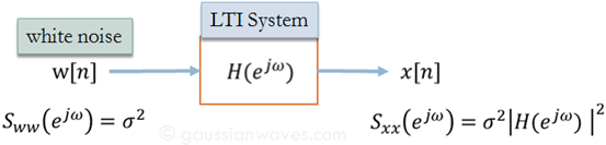
Motivation: We want to describe the PSD of a signal $x[n]$ with the following model. In this way we can describe the signal $x[n]$ only with the parameters of the LTI system and thus reduce the burden of communication system.
- Autoregressive model (AR) : Sum of past $x[n-k]$ + current source input $\omega [n]$
where $a_i, … ,a_N$ are the parameters of the model and $\omega [n]$ is the source input white noise.
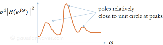
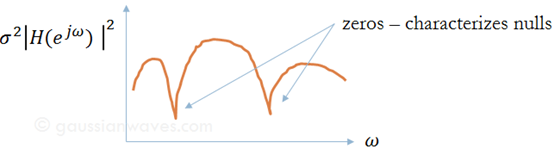
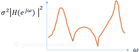
The frequency response of the IIR filter is well known: $H(e^{jω})$ is an all-poles system
The PSD of $x[n]$ is:
- Moving-average model (MA) : Sum of past and current source inputs i.i.d. $\omega[n-k]$
where the $b_0,…,b_M$ are the parameters of the model and the $\omega[n], \omega[n-1], …, \omega[n-M]$ are i.i.d. source inputs. video
The frequency response of the FIR filter is well known: $H(e^{jω})$ is an all-zeros system
The PSD of $x[n]$ is:
- Autoregressive–moving-average model (ARMA) :
The frequency response of this generalized filter is well known: $H(e^{jω})$ is an pole-zero system
The PSD of $x[n]$ is:
Introduction of Estimation Theory
Estimation in signal processing
Mathematically, we have the $N$-point data set ${x[0], x[1], … , x[N-1]}$ which depends on an unknown parameter $\theta$. We wish to determine $\theta$ based on the data or to define an estimator
where $g$ is some function. This is the problem of parameter estimation.
class note: what is $\hat{\theta}?$Since $X$ is a random variable, the estimation $\hat{\theta}$ is also a random variable. However, the time series ${x[0], x[1], … , x[N-1]}$ is a sample of $X$ and thus $\hat{\theta}$ gained from the $g$ is a deterministic estimation. It is pretty important to bear in mind that every estimation based on specific input-output is only a sample.
If we can improve the performance of random variable $\boldsymbol{\hat{\theta}}$, when we dealing with deterministic signals, we are more likely to gain a better deterministic estimation.
The mathematical estimation problem
In determining good estimators, the first step is to mathematically model the data. Because the data are inherently random, we describe it by its probability density function (PDF) or $\mathbf{p(x[0], x[1], … , x[N-1];\boldsymbol\theta)}$
If we have prior knowledge Bayesian Estimation is a probable method and we describe the data by joint PDF:
where $p(\theta)$ is the prior PDF, summarizing our knowledge about $\theta$ before any data are observed, and $p(x|\theta)$ is a conditional PDF, summarizing our knowledge provided by the data $\mathbf{x}$ conditioned on knowing $\theta$.
class note: the notation of probability $f(x;\theta)$, $f(x,\theta)$ and $f(x|\theta)$$f(x;\theta)$ is the density of the random variable $X$ at the point $x$, with $\theta$ being the parameter of the distribution. $f(x,\theta)$ is the joint density of $X$ and $\Theta$ at the point $(x,\theta)$ and only makes sense if $\Theta$ is a random variable. $f(x|\theta)$ is the conditional distribution of $X$ given $\Theta$, and again, only makes sense if $\Theta$ is a random variable. This will become much clearer when you get further into the book and look at Bayesian analysis.
$f(x; \theta) \approx f(x,\theta)$ in this course.
Minimum Variance Unbiased Estimation
MVU is a standard of an effective estimation.
It includes two parts: Unbiased and Minimum Variance
It is the goal of our methods for estimation.
Specific methods to reach to MVU are presented in latter chapters.
class note: Why mean+variance is sufficient?This is because $\hat{\theta}$ is often generated by linear equations, with Central limit theorem, $\hat{\theta}$ is similar to a gaussian variable. This is the reason why we only need mean, 1st statistic, and variance, 2nd statistic, to evaluate $\hat{\theta}$.
Unbiased estimation
Since the parameter value may in general be anywhere in the interval $a < \theta < b$, unbiasedness asserts that no matter what the true value of $\theta $, our estimator will yield it on the average.
Minimum Variance Criterion
In searching for optimal estimators we need to adopt some optimality criterion. A natural one is the mean square error (MSE):
This measures the average mean squared deviation of the estimator from the true value. Unfortunate, adoption of this natural criterion leads to unrealizable estimators, and so we rewrite the MSE as
Minimum Variance Unbiased Estimation is to constrain the bias to be zero and find the estimator which minimizes the variance.
Cramer-Rao Lower Bound
class note: why we need CRLB?From the last chapter, we know that a better estimation will have lower variance. CRLB provides the lower band of this variance and it becomes the objective of designs of algorithms.
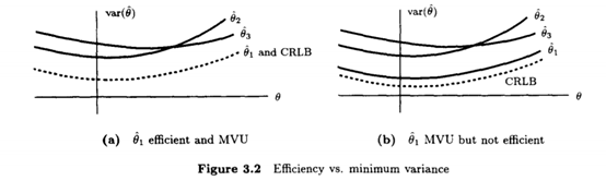
Efficiency
An estimator which is unbiased and attains the CRLB is said to be efficient in that it efficiently uses the data. An MVU estimator may or may not be efficient.
Scalar parameter
Theorem (Cramer-Rao Lower Bound - Scalar Parameter)
1)
It is assumed that the PDF $p(\mathbf{x};\theta)$ satisfied the “regularity” condition
where the expectation is taken with respect to $p(\mathbf{x};\theta)$. Then, the variance of any unbiased estimator $\hat{\theta}$ must satisfy
where the derivative is evaluated at the true value of $\theta$ and the expectation is taken with respect to $p(\mathbf{x};\theta)$.
2)
The denominator is referred to as the Fisher information:
The more information, the lower the bound.
3)
Furthermore, an unbiased estimator may be found that attains the bound for all $\theta$ if and only if
for some functions $g$ and $I$. That estimator, which is the MVU estimator, is $\hat{\theta}=g(\mathbf{x})$, and the minimum variance is $1/I(\theta)$.
Scalar parameter · transformation
Situation: The parameter we wish to estimate is a function of some more fundamental parameter.
Although efficiency is reserved only over linear transformations, it is approximately maintained over nonlinear transformations if the data record is large enough (Asymptotic efficiency). This has great practical significance in that we are frequently interested in estimating functions of parameters.
Given the transformation: $g(\theta)=a\theta +b$
Step1: Estimate single parameter $\hat{\theta}$.
Step2: $\widehat{g(\theta)}=g(\hat{\theta})=a\hat{\theta}+b$
Vector parameter
Theorem (Cramer-Rao Lower Bound - Vector Parameter)
1)
It is assumed that the PDF $p(\mathbf{x}; \boldsymbol \theta)$ satisfies the “regularity” conditions:
where the expectation is taken with respect to $p(\mathbf{x}; \boldsymbol \theta)$. Then, the covariance matrix of any unbiased estimator $\boldsymbol{ \hat{\theta}} $ satisfies:
where $\geq\mathbf 0$ is interpreted as meaning that the matrix is positive semidefinite.
In probability theory and statistics, a covariance matrix is a matrix whose element in the i,j position is the covariance between the i-th and j-th elements of a random vector. A random vector is a random variable with multiple dimensions. Each element of the vector is a scalar random variable.
A $n \times n$ symmetric real matrix $\displaystyle M$ is said to be positive semidefinite or non-negative definite if ${\displaystyle x^{\textsf {T}}Mx\geq 0}$ for all non-zero ${\displaystyle x}$ in ${\displaystyle \mathbb {R} ^{n}}$ . Formally,
2)
$\mathbf{I}(\boldsymbol\theta)$ is the $p\times p$ Fisher information matrix. The latter is defined by:
$\mathbf{I}^{-1}$ exists $\Leftrightarrow$ $rank(\mathbf{I})=p$
If $rank(\mathbf{I})\prec p$, we can’t estimate an efficient channel. e.g. If $rank(\mathbf{I})=p-1$, we require a known parameter.
3)
Furthermore, an unbiased estimator may be found that attains the bound in that $\mathbf{C_{\boldsymbol{ \hat{\theta}}}}=\mathbf{I}^{-1}(\boldsymbol {\theta})$ if and only if
for some p-dimensional function $\mathbf g$ and some $p \times p$ matrix $\mathbf I$. That estimator, which is the MVU estimator, is $\boldsymbol {\hat {\theta}} = \mathbf g(\mathbf{x})$, and its covariance matrix is $\mathbf{I}^{-1}(\boldsymbol {\theta})$.
Vector parameter · transformation
Similar to “Scalar parameter · transformation”.
Linear Model
class note: why we need Linear Model?The determination of the MVU estimator is in general a difficult task. It is fortunate, however, that a large number of signal processing estimation problems can be represented by a data model that allows us to easily determine this estimator. This class of models is the linear model.
Linear model · specific
Theorem (Minimum Variance Unbiased Estimator for the Linear Model)
If the data observed can be modeled as
where $\mathbf{x}$ is an $N \times 1$ vector of observations, $\mathbf H$ is a known $N\times p$ observation matrix (with $N\succ p$) and rank p, $\boldsymbol \theta$ is a $p\times1$ vector of parameters to be estimated, and $\mathbf w$ is an $N\times1$ noise vector with PDF $N(\mathbf 0, \sigma^2 \mathbf I)$, then the MVU estimator is
and the covariance matrix of $\boldsymbol{\hat{\theta}}$ is
For the linear model the MVU estimator is efficient in that it attains the CRLB.
Linear model · general
A more general form of the linear model allows for noise that is not white. The general linear model assumes that
where $\mathbf C$ is not necessarily a scaled identity matrix. The MVU estimator is
The biggest difference with “Linear model · white noise” is that the estimator requires statistics of the noise. The covariance matrix of $\boldsymbol{\hat{\theta}}$ is
For the general linear model the MVU estimator is efficient in that it attains the CRLB.
class note: Serial channel estimation using linear modelThis method is based on Training sequence.
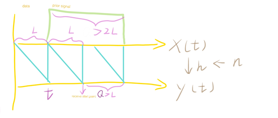
The receive signals start at $t+L$ because we should make sure that our $y$ is totally derived from prior signal instead of data.
$L$ is the channel latency, $S$ is the prior signal with length of $Q$. Then we can build a linear model to gain the MVU estimator:
$\left[
\begin{matrix}
S
\end{matrix}
\right]$ is a matrix with $s(t)$ components.
There are three rules:
- The length of prior signal $\geq$ $2L-1$. To enhance performance, the length should increase.
$\mathbf{H}$ requires to be full column rank and thus we should better design the prior signal $s$.
$\mathbf{H}^T\mathbf{H}=C \cdot \mathbf{I}$ is the best choice because $\mathbf{H}^T\mathbf{H}$ has uniform eigenvalues so its inverse will not enlarge the $\mathbf{N}$.
In an OFDM system, we can estimate its channel based on pilot sequence in frequency domain and linear model. The length of signals in each step are shown as follow:

The whole system can be described as:
$M$ is the length of original signal, $N$ is the length of pilot sequences and $L$ is the length of channel. Then we can build a linear model to gain the MVU estimator:
$P$ is the pilot sequence and $\left[
\begin{matrix}
S
\end{matrix}
\right]$ is the combination of $e^{-j\frac{2\pi}{L}kl}$ and $S(k)$.
Maximum Likelihood Estimation
Scalar parameter
The MLE for a scalar parameter is defined to be the value of $\theta$ that maximizes $p(\mathbf{x};\theta)$ for $\mathbf{x}$ fixed, i.e., the value that maximizes the likelihood function.
The method defines a maximum likelihood estimate:
if a maximum exists.
Relation to Bayesian inference:
The maximum a posteriori estimate:Bayes’ theorem:
when the prior $p(\theta)$ is a uniform distribution, MAP is the same as MLE.
Theorem 1 (Asymptotic Properties of the MLE):
From the asymptotic distribution, the MLE is seen to be asymptotically unbiased and asymptotically attains the CRLB. It is therefore asymptotically efficient, and hence asymptotically optimal.
Theorem 2 (Invariance Property of the MLE)
Similar to “Cramer-Rao Lower Bound/ Scalar parameter · transformation”
The MLE of the parameter $\alpha = g(\theta)$, where the PDF $p(\mathbf{x}; \theta)$ is parameterized by $\theta$, is given by
where $\hat{\theta}$ is the MLE of $\theta$.
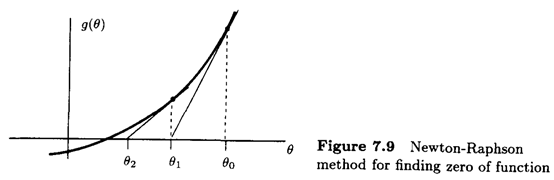
Numerical determination
We attempt to solve the equation:
Then, if $g(\theta)$ is approximately linear near $\theta_0$, we can approximate it by (Taylor series):
Least Squares
Linear Least Squares
In applying the linear LS approach for a scalar parameter we must assume that
where $h[n]$ is a known sequence and $s[n]$ is a purely deterministic signal. Due to observation noise or model inaccuracies we observe a perturbed version of $s[n]$, which we denote by $x[n]$. The LS error criterion becomes
A minimization is readily shown to produce the LSE
This equation is similar to $\frac{R(xy)}{R(yy)}$ in channel estimation.
class note: Conclusion of estimation methodsCRLB:
Condition:
- know the PDF $p(\mathbf{x};\theta)$
- the “regularity” condition $E[\frac{\partial \ \ln p(\mathbf{x};\theta)}{\partial \theta}]=0 \ \ \ \ for\ all\ \theta$
Estimator: if $ \frac{\partial \ \ln p(\mathbf{x};\theta)}{\partial \theta}=I(\theta)(g(\mathbf{x})-\theta) $
- Scalar parameter: efficient (MVU)
- Vector parameter with full rank: efficient (MVU)
- Vector parameter without full rank: inefficient
- Scalar / Vector parameter · transformation: asymptotically efficient
Linear Model:
Condition:
- know the PDF $p(\mathbf{x};\theta)$
- the distribution is gaussian
- can use the form: $\mathbf x = \mathbf H \boldsymbol \theta + \mathbf w$
Estimator:
- specific / general: efficient (MVU)
MLE:
Condition:
- know the PDF $p(\mathbf{x};\theta)$
- Estimator:
- if $p(\mathbf{x};\theta)$ is gaussian, then MVU
- if $p(\mathbf{x};\theta)$ is not gaussian, then asymptotically efficient and asymptotically MVU
- LSE:
- Condition:
- none
- Estimator:
- if $p(\mathbf{x};\theta)$ is gaussian, then efficient (MVU)
- if $p(\mathbf{x};\theta)$ is not gaussian, then whether it’s MVU is unclear because we don’t have statistics of $\mathbf{x}$
- Condition:
Statistical detection theory
Our intention is to do a binary hypothesis testing
- $P(H_0;H_0)$ = prob(decide $H_0$ when $H_0$ is true) = prob of correct non-detection
- $P(H_0;H_1)$ = prob(decide $H_0$ when $H_1$ is true) = prob of missed detection = $P_M$
- $P(H_1;H_0)$ = prob(decide $H_1$ when $H_0$ is true) = prob of false alarm = $P_{FA}$
- $P(H_1;H_1)$ = prob(decide $H_1$ when $H_1$ is true) = prob of detection = $P_D$
Neyman-Pearson Theorem
Condition: None
To maximize $P_D$ for a given $P_{FA}=a $ , decide $H_1$ if:
where the threshold $\gamma$ is found from:
$L(x)$ is the likelihood ratio , and comparing $L(x)$ to a threshold is termed the likelihood ratio test.
Minimum Probability of Error
Condition: Priors $P(H_0), P(H_1)$
Assume that we know the prior probability $P(H_0)$ and $P(H_1)$, our goal is to minimize the probability of error $P_e $ :
It is a special case of Bayes Risk. So the estimator is to decide $H_{1}$ if:
Bayes Risk
Condition: Priors $P(H_0), P(H_1)$ & Costs $C_{ij}$
Associate with each of the four detection possibilities a cost. $C_{ij}$ is the cost of deciding hypothesis $H_i$ when hypothesis $H_j$ is true.
Under the assumption that $C_{10}>C_{00}$ , $C_{01}>C_{11}$ , the detector that minimizes the Bayes risk is to decide $H_{1}$ if:
Minimax Hypothesis Testing
Condition: Costs $C_{ij}$
In general, no single decision rule minimizes the Bayes risk over all possible $P(H_{i/j})\in [0, 1]$. Our intention is to avoid possible huge risk so we try to minimize the maximum loss.
Minimax Hypothesis Testing Formulation:
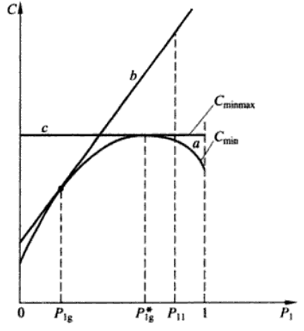
“a” is the minimum Bayesian risk when $P(H_{1}) \in [0,1]$. Once we assume that the prior probability $P(H_1)=P_{1g}$, $P_{FA}$ and $P_M$ are known. and “a” will be reshaped as “b”, which may leads to huge risk when the exact $P_{1}$ is far different from $P_{1g}$.
Minimax Hypothesis Testing tends to assume that $P(H_1)=P_{1g}^{*}$.